Using math software for teaching calculus

I have been teaching for seven years now. Yet somehow, I started only recently using computer algebra software (CAS) to make live illustrations of mathematical concepts in class. And I have to say that it is quite useful!

Previous attempts

As you may know, I am/was a big proponent of free software, so I had only ever used tools like SageMath or Julia. However, to be honest, I always found them relatively lackluster for what I had in mind (no offense meant to the developers of these tools!). I found that performing even simple tasks was quite convoluted. For example, here is how you find the roots of the polynomial $x^3 - 1$ in SageMath, taken directly from the documentation:

x = PolynomialRing(RationalField(), 'x').gen()
f = x^3 - 1
f.roots()
# [(1, 1)]
f = (x^3 - 1)^2
f.roots()
[(1, 2)]
x = PolynomialRing(CyclotomicField(3), 'x').gen()
f = x^3 - 1
f.roots()
# [(1, 1), (zeta3, 1), (-zeta3 - 1, 1)]

Factoring this polynomial thus requires me to already know that the splitting field is the third cyclotomic field. This kinda defeats the purpose. Moreover, it means that I just cannot tell first-year undergrads to do it on their own. And if I show them my code, I can only tell them that the line:

x = PolynomialRing(CyclotomicField(3), 'x').gen()

is a magic command that allows me to factor this specific polynomial. And if they want to understand it – let alone apply it to other examples – they’ll have to wait for a couple of years and a proper Algebra class.

There was moreover, in my opinion, a real problem with documentation (especially with SageMath, which is the “big player” of the field). Most of it is written in the form of examples. This is fine to get the hang of how to use a particular function. However, as soon as you want to use more advanced features, or configure different options than what is provided in the examples, you’re out of luck. A colleague told me that most of SageMath’s documentation is actually a suite of unit tests. While this could make sense from a developer’s perspective, from a user’s point of view, this is subpar.

Mathematica

After learning that my university had a site-wide license for Mathematica, I decided to give it a try. Even though I learned about Maple during my undergrad, Mathematica sounded appealing due to its handling of rewriting rules, which is directly relevant to some of my research projects. I was also intrigued by the language, which I have seen described as a “weird kind of Lisp.” And finally, well, I am a researcher, so I’m curious at heart and I always want to learn new things and I plunged in.

The user interface of Mathematica is based on notebooks, and I am told that this concept was actually popularized by Mathematica. I was already familiar with notebooks, which I used e.g., in my intro to algorithms class. In short, a standard Mathematica file is made out of many “cells.” Each cell can either contain code, which can be executed, or text, which can be formatted. The text cells can be headings for chapters, sections, etc., or they can be plain-text explanations of the surrounding code. Code cells are further subdivided into an input cell, which contains the code to be executed, and an output cell, which contains the result. Cells can be moved around in the document, executed out of order… The end result looks like this:

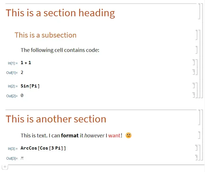
In what follows, I will only include the code (which follows lines starting with In[...]:=) and the result given by Mathematica (starting with Out[...]=). For example, the code of the previous screenshot reads:

In[1]:= 1 + 1
Out[1]= 2

In[2]:= Sin[Pi]
Out[2]= 0

In[3]:= ArcCos[Cos[3Pi]]
Out[3]= \[Pi]

Mathematica’s syntax is somewhat unusual, as you can already see in the above example.

• Function application is written with square brackets; parentheses are only used for grouping. For example, f[x] is the application of the function f to the variable x, whereas f(x) is the multiplication of f with x.
• Built-in functions and objects all have names that start with an uppercase letter (e.g., Sin or Pi). The code is case-sensitive; if I had written sin[pi], Mathematica wouldn’t have known what to do with it.
• There is extensive support for graphical formulas, as I explain below.

Graphical formulas

When I asked Mathematica to compute $\operatorname{arccos}(\cos(3\pi))$ (by inputting ArcCos[Cos[3Pi]]), it answered with $\pi$ written as the Greek letter, not written as its spelled out English name Pi. This is known as the “Standard Form” representation of the formula. When I copy-pasted it as plain text in the Markdown document that I am currently writing, it got converted into a plain-text representation of the Greek letter $\pi$, which is internally represented in Mathematica by \[Pi].

I am also able to ask Mathematica to display the result in “Input Form,” i.e., a form which is suitable for entering on a standard English (or French) keyboard. When I ask Mathematica to do that, it transforms the $\pi$ (internally represented as \[Pi]) into Pi, which is how I typed it in the input cell In[3].

For traditionalists, there is also something called the “Traditional Form”, which resembles more closely traditional mathematical notation. Converting ArcCos[Cos[3Pi]] into traditional form yields $\cos^{-1}(\cos(\pi))$, which is how I could hand-write the formula if I weren’t French and didn’t prefer $\operatorname{arccos}$ to $\cos^{-1}$. However, traditional form is ambiguous: for example, a 2-by-1 matrix of integers surrounded by parentheses $\left( \begin{smallmatrix} n \\ k \end{smallmatrix} \right)$ could just as easily be interpreted as a binomial coefficient $\binom{n}{k}$. Mathematica does its best to interpret it, but this shouldn’t be relied upon.

It’s possible to actually input graphical formulas, rather than just displaying them as output. There is also a long list of keyboard shortcuts that makes inputting graphical formulas easier. For example, if I want to write a polynomial, I can decide to write it like this:

In[4]:= Sum[Subscript[a, i]*x^i, {i, 0, 5}]
Out[4]= Subscript[a, 0] + x Subscript[a, 1] + x^2 Subscript[a, 2] + x^3 Subscript[a, 3] + x^4 Subscript[a, 4] + x^5 Subscript[a, 5]

(Inside Mathematica’s frontend, the output doesn’t literally display Subscript[a, 3], for example, but rather $a_3$ as you would expect.) But I can also, using a couple of shortcuts for subscripts/superscripts and inputting the “sum” character $\sum$ as Esc sum Esc, input it like this:

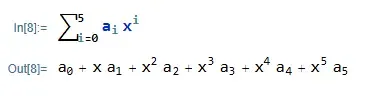
This makes for concise and nice-looking formulas, in my opinion.

The old example

Getting back to my earlier example about factoring $x^3-1$, this becomes:

In[5]:= Factor[x^3 - 1]
Out[5]= (-1 + x) (1 + x + x^2)

In[6]:= Factor[x^3 - 1, Extension -> All]
Out[6]= (-1 + x) ((-1)^(1/3) + x) (-(-1)^(2/3) + x)

Without all of SageMath’s ceremonial or pre-guessing of the splitting field.

Documentation

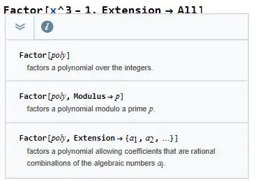
The documentation is also stellar. Let’s say I want to learn more about the Factor function from before. The first thing I can do is hover with my mouse over the word Factor in the formula. I am then presented with a little pop-up that can either show me a quick help window with basic information on how to use the function:

Or I can click on the information button (or alternatively, press F1 when my cursor is on the word Factor), and I get taken to the full help page for the function. This help page is available online here. As you can see, it is very complete: it contains example usage, a full list of options, what they mean and how they can typically be used, a list of advanced examples (under “Scope” or “Applications”), and even a section with “Neat examples” that often contains nice illustrations.

What is particularly nice is that the whole documentation is included in Mathematica in the form of a notebook. And this notebook is writable! So if you see an example and wonder what happens if you modify it slightly, well, you can just start typing/modifying it, and run it instantly inside Mathematica. No more back and forth or copy-paste between the documentation and the software. There is also a list of related help topics that link to other places in the documentation and has been a great help from time to time. The word I find describes best the user interface is “smooth.”

A concrete example

In my calculus course, one concept I had to teach was the difference between continuity and uniform continuity (for real functions of one real variable). As you all know, a real map $f : I \to \mathbb{R}$ defined on an interval $I \subseteq \mathbb{R}$ is continuous when:

$$\forall x \in I, \forall \epsilon > 0, \exists \delta > 0, \forall y \in I, \quad |x-y| < \delta \implies |f(x) - f(y)| < \epsilon.$$

On the other hand, $f$ is uniformly continuous if:

$$\forall \epsilon > 0, \exists \delta > 0, \forall x \in I, \forall y \in I, \quad |x-y| < \delta \implies |f(x) - f(y)| < \epsilon.$$

This difference in definitions is a nice example to teach students that when you change the order of quantifiers, you get a different statement. In particular, they should always write a quantifier (either symbolically or in a sentence such as “For any $x$, …”) instead of starting to write statements about variables that were not introduced before 🙂. (This is one of my life-long struggle as a math teacher, I guess.)

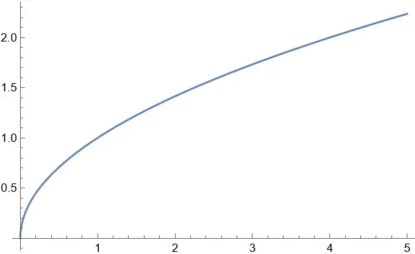
Let’s take the example of the square root, $f : [0, +\infty) \to \mathbb{R}$, $x \mapsto \sqrt{x}$. This one is, of course, uniformly continuous. How can I illustrate that with Mathematica? First, here’s the plot of the map produced by Mathematica (with the command Plot[Sqrt[x], {x, 0, 1}])

Well, I can actually just ask Mathematica to find the $\delta$ given the $\epsilon$!

Continuity at a point

First, I can ask it to find a value of $\delta$ for a fixed $a \ge 0$, as follows:

In[1]:= continuity[a_] =
 Reduce[{ε > 0, δ > 0, a >= 0,
  ForAll[x, x >= 0,
   Implies[Abs[x - a] < δ,
    Abs[Sqrt[x] - Sqrt[a]] < ε]]}, δ, Reals]

Out[1]= ε > 0 &&
  ((0 <= a < ε^2 &&
     0 < δ <= ε^2 +
       2 Sqrt[a ε^2]) || (a == ε^2 &&
     0 < δ <= a) || (a > ε^2 &&
     0 < δ <= -ε^2 + 2 Sqrt[a ε^2]))

I am not sure that the plain-text representation does justice to the formula, so here is yet another screenshot:

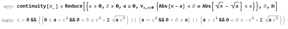
What did I do here? The Reduce function “reduces” a logical statement to a simpler one. Here, I asked Mathematica to reduce the following statement, to give me the answer in terms of conditions on $\delta$, assuming every parameter is real:

$$\epsilon > 0 \land \delta > 0 \land a \geq 0 \land \forall x \geq 0, (|x-a| < \delta \implies |\sqrt{x}-\sqrt{a}| < \epsilon).$$

Since I ask the answer to be in terms of $\delta$, the parameters $\epsilon$ and $a$ are implicitly written with a $\forall$ in front of them. This is of course the statement that says “the square root is continuous at $a$.” And Mathematica answered that $\epsilon$ must be positive (obviously, it’s one of the assumptions), and that there are three cases:

• If $a < \epsilon^2$, then we must have $\delta < \epsilon^2 + 2 \sqrt{a \epsilon^2}$;
• If $a = \epsilon^2$, then we must have $\delta < \epsilon^2$;
• If $a > \epsilon^2$, then we must have $\delta < -\epsilon^2 + 2 \sqrt{a \epsilon^2}$.

This is something that you can check by hand. It is rather painful to do on paper, but Mathematica did it almost instantly. Isn’t that great?

I can also visualize the answer using the following command, which tells Mathematica “plot the region defined by continuity[a] for $0 \leq \delta \leq 3$ and $0 \leq \epsilon \leq 1$, with the parameter $a$ varying between $a=0$ and $a=1$:

Manipulate[
 RegionPlot[
  continuity[a], {δ, 0, 3}, {ε, 0, 1}],
 {{a, 1}, 0, 1}]

And the result is (with the video produced by Mathematica’s own Export command):

Uniform continuity

Now, what about uniform continuity? Can I ask Mathematica to find a value of $\delta$ that works for all possibles values of $a$? Sure can do! The answer is another call to Reduce:

In[3]:= Reduce[{ε > 0, δ > 0,
  ForAll[a, a >= 0,
   ForAll[x, x >= 0,
    Implies[Abs[x - a] < δ,
     Abs[Sqrt[x] - Sqrt[a]] < ε]]]}, δ]

Out[3]= ε > 0 && 0 < δ <= ε^2

I told Mathematica to find (in terms of $\delta$, with an implicit $\forall$ for the other parameters) a statement logically equivalent to:

$$\epsilon > 0 \land \delta > 0 \land \forall a, x \geq 0, |x-a| < \delta \implies |\sqrt{x} - \sqrt{a}| < \epsilon.$$

This is of course the statement that says that the square root is uniformly continuous. And Mathematica answered: $\delta$ needs to be at most $\epsilon^2$. Since a solution exists, the map is uniformly continuous. And I can visualize this with another call to Manipulate

In blue, you can see the same region as before: for a given value of $a$, what values of $(\delta, \epsilon)$ make the statement true? In orange, this is the region for the uniform continuous: the couples $(\delta,\epsilon)$ that make the statement true regardless of the actual value of $a$. You can roughly see that this orange region is, indeed, the (nonempty) intersection of all the blue regions.

A counterexample

And to finish this post, let us illustrate with a map which is not uniformly continuous, namely, $f(x) = 1/x$ (defined on e.g., positive reals). Again, a call to Reduce allows me to know what values of $\delta$ work given $a$ and $\epsilon$:

In[7]:= continuity2[a_] =
 Reduce[{ε > 0, δ > 0, a > 0,
   ForAll[x, x >= 0,
    Implies[Abs[x - a] < δ,
     Abs[1/x - 1/a] < ε]]}, δ]

Out[7]= ε > 0 && a > 0 && 0 < δ <= (a^2 ε)/(1 + a ε)

So $\delta$ can be at most $\frac{a^2 \epsilon}{1+a\epsilon}$. What happens when $a$ ranges over all possible values, rather than taking on a fixed value?

In[8]:= Reduce[{ε > 0, δ > 0,
  ForAll[a, a >= 0,
   ForAll[x, x >= 0,
    Implies[Abs[x - a] < δ,
     Abs[1/x - 1/a] < ε]]]}, δ]

Out[8]= False

Mathematica reduced the statement to a simpler one. The statement is false, as expected! The map $x \mapsto 1/x$ is not uniformly continuous.